Molecular Visualization with v, vmol, and xyzrender
Molecular Visualization with v, vmol, and xyzrender
This guide covers a lightweight Linux/WSL workflow for looking at molecular structures and making clean 2D figures:
-
v— a fast X11 molecular viewer (rotate, animate modes, dump reoriented XYZ). -
vmol— the Python package / CLI wrappers aroundv(vmol,vmol2). -
xyzrender— publication-quality SVG/PNG/PDF renders from XYZ, cube files, and many QM outputs; usesvmol/vfor interactive orientation.
By the end you should be able to open a structure from the terminal, orient it interactively, render a figure from the CLI or a Jupyter notebook, and build multi-style images (for example a Paton ball-and-stick adsorbate on a vdW metal slab) like the camphor/Cu(111) and bipyridine/Au(111) panels used in our surface papers.
If Conda/environments are unfamiliar, start with Local Conda and VS Code Setup. For basic shell skills, see Linux Sysadmin Basics.
How the pieces fit together
| Tool | Role | Needs a display? |
|---|---|---|
v / vmol
|
Interactive 3D viewing (X11) | Yes (unless headless gui:0) |
vmol2 |
Same viewer, but loads ORCA/Gaussian/… via cclib
|
Yes |
xyzrender |
Static figures (SVG/PNG/PDF) and notebook inline display | No for plain renders; yes for -I / orient()
|
Typical figure workflow: open the molecule in vmol (or xyzrender -I), rotate to a useful view, press z to emit XYZ, then let xyzrender draw the publication graphic.
1. Prerequisites: X11 on Linux and WSL
v/vmol draw with X11. Plain SVG/PNG rendering with xyzrender does not need a display.
Native Linux
Most desktop installs already have X11. From a graphical session, echo $DISPLAY should print something like :0 or :1. If you SSH into a remote machine, use X11 forwarding (ssh -X / ssh -Y) or run the viewer locally on files you copy back.
WSL (Windows Subsystem for Linux)
-
Windows 11 + WSLg: GUI apps usually work out of the box. In Ubuntu/WSL, check
echo $DISPLAY(often:0). -
Windows 10 / no WSLg: install an X server on Windows (VcXsrv, X410, …), start it, then in WSL set e.g.
export DISPLAY=:0(or the address your X server documents). - Run these tools from a WSL terminal, not from native Windows PowerShell — the packages are Linux wheels.
If vmol exits immediately or complains about opening a display, fix the DISPLAY variable or the X server first — it is almost never a Python problem.
2. Install in a Conda (or venv) environment
Activate the environment you use for notebooks / chemistry scripts, then:
# Interactive viewer + xyzrender (recommended on Linux/WSL)
pip install 'xyzrender[v]'

# Or install the pieces separately:
# pip install vmol          # v wrapper (XYZ / Priroda)
# pip install 'vmol[all]'   # + cclib → vmol2 for ORCA/Gaussian logs
# pip install xyzrender     # figures only (no interactive v)
Quick checks:
vmol -h          # or: vmol   (no args → help / reference)
xyzrender -h
python -c "import vmol, xyzrender; print('ok')"
vmol ships manylinux wheels for current CPython versions. Building from source is documented in the vmol install notes if you need a custom v.so.
3. CLI: view structures with vmol
Native XYZ (and Priroda) files:
vmol molecule.xyz
Useful options (same language as upstream v):
vmol molecule.xyz bonds:0              # hide bonds
vmol molecule.xyz colors:cpk           # CPK colors (default scheme is colors:v)
vmol crystal.xyz cell:10,10,10         # cubic cell in Å
vmol traj.xyz dt:0.05                  # slower frame delay
ORCA / Gaussian / other outputs that v does not read natively — use vmol2 (needs cclib):
pip install 'vmol[all]'   # if you have not already
vmol2 job.out             # ORCA
vmol2 job.log             # Gaussian
vmol2 job.log vib:0       # force geometry frames instead of normal modes when both exist
You can also run the modules explicitly:
python -m vmol molecule.xyz
python -m vmol.vmol2 job.out
Essential keyboard shortcuts
| Key | Action |
|---|---|
| mouse / arrows | rotate (Ctrl/Shift = slower) |
Home / End
|
zoom in / out |
n / t / l / b
|
toggle numbers / types / bond lengths / bonds |
Enter / Backspace
|
next / previous frame |
Ins |
play animation / vibrate selected mode |
z |
print current geometry as XYZ (stdout) |
x |
print Priroda-style input |
p |
print input aimed at SVG generators |
u |
print rotation matrix |
m |
save current frame as .xpm
|
q / Esc
|
quit |
Full tables live in the v README.
Orient once, then render (pipe)
vmol molecule.xyz | xyzrender -o molecule.svg
Rotate in the viewer, press z (the XYZ goes into the pipe), then q. xyzrender reads stdin and writes the figure. Auto-orientation is off when input comes from stdin.
4. CLI: figures with xyzrender
Basic XYZ → SVG (auto-oriented by default):
xyzrender caffeine.xyz
xyzrender caffeine.xyz -o figure.png
xyzrender caffeine.xyz -o figure.pdf --hy --config paton
From QM outputs (format auto-detected):
xyzrender calc.out
xyzrender calc.out --ts          # emphasize TS-like bonds when supported
Interactive orientation, then render (opens vmol by default):
xyzrender molecule.xyz -I -o oriented.svg
xyzrender molecule.xyz -I --viewer vmol -o oriented.png
In the viewer: rotate → z → q/Esc. Reuse a saved orientation across related files with --ref (see the orientation docs).
5. Python notebooks
Install the same packages into the kernel’s environment, then:
from xyzrender import load, render, orient

mol = load("caffeine.xyz")
render(mol)                              # inline SVG in Jupyter
render(mol, output="caffeine.svg")       # also write a file
render(mol, hy=True, config="paton")
Interactive orientation from the notebook (needs a working X11 display — fine on Linux desktops and WSL with WSLg):
orient(mol)                              # opens vmol; rotate, press z, then q
render(mol, output="oriented.svg")       # uses the locked orientation
GIFs:
from xyzrender import render_gif

render_gif(mol, gif_rot="y", output="spin.gif")
Cube / surface examples (when you have .cube data):
mol = load("orbital.cube")
render(mol, mo=True, iso=0.05)
Calling vmol directly from Python
For scripts that only need the viewer / captured XYZ (without xyzrender):
from vmol import vmol

# Open interactively
vmol.run(["molecule.xyz"])

# Rotate, press z (or x/p), then q — capture printed text
out = vmol.capture(args=["molecule.xyz"])
print(out)

# Pass coordinates without a file (numpy-friendly)
out = vmol.capture(
    mols={"q": [1, 9], "r": [[0.0, 0.0, 0.0], [0.92, 0.0, 0.0]], "name": "HF"},
    args=["shell:0.6,0.7"],
)
ASE Atoms objects and multi-frame lists are supported as mols=; see the vmol examples.
Headless point-group check (no window):
from vmol import vmol

print(vmol.capture(args=["molecule.xyz", "gui:0", "com:."]))
6. Multi-style figures: Paton molecule + vdW slab
Uniform presets are fine for organics. Surface adsorption figures usually need two styles in one image:
-
Adsorbate →
paton(clean PyMOL-like ball-and-stick; carbons often pale). -
Metal slab →
vdw(opaque space-filling spheres so the lattice reads as a surface).
xyzrender supports this with style regions: a base --config for most atoms, plus --region (CLI) or regions= (Python) for atom subsets. Official overview: Style Regions.
Target look (from our camphor/Cu and bipyridine/Au figure pipelines):
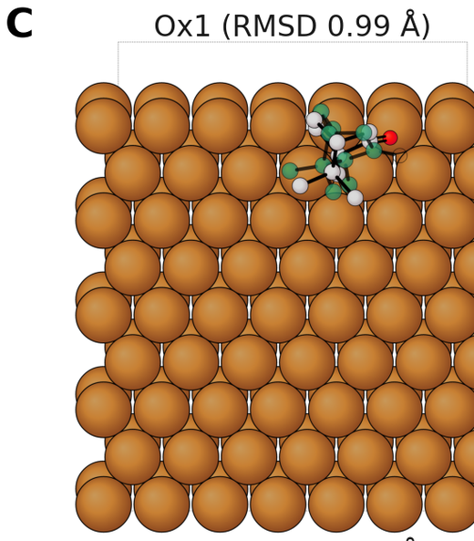
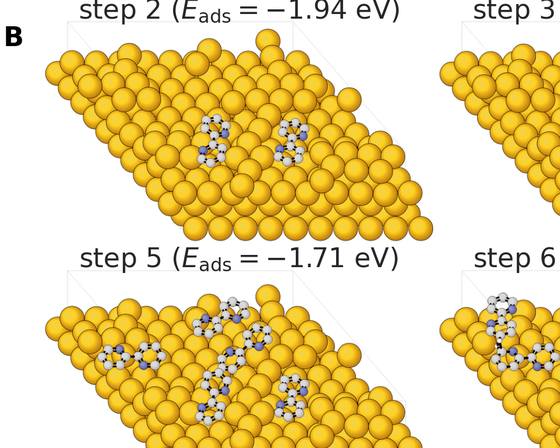
6.1 Presets alone (why regions matter)
Same toy slab+molecule XYZ, three uniform choices:
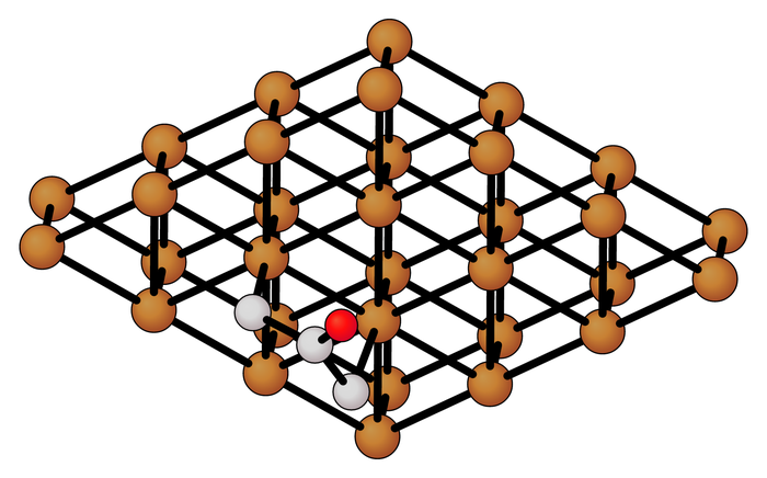
--config paton everywhere — slab bonds clutter the surface.
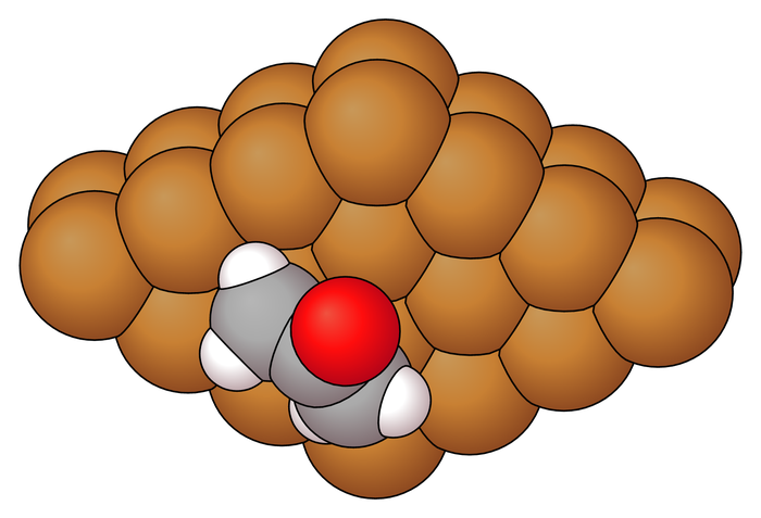
--config vdw everywhere — adsorbate connectivity disappears into spacefill.
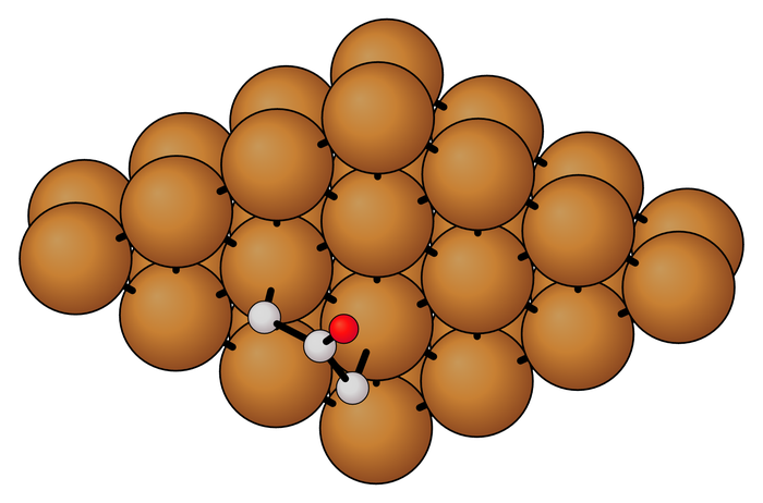
paton + metal vdw region — the style used for camphor/bipyridine panels.
6.2 CLI recipe
Atom selectors are 1-indexed. You can use index ranges ("1-32"), elements ("Cu", "Au", "Pt"), or categories ("M" for metals).
# Metals (element selector) as vdW; everything else keeps the base Paton style
xyzrender slab_adsorbate.xyz \
  --config paton \
  --region "Cu" vdw \
  --unbond Cu-Cu --unbond Cu-C --unbond Cu-O --unbond Cu-H \
  --no-orient \
  -o figure.png
Notes:
-
--region ATOMS CONFIGis repeatable (several fragments, several styles). -
--unbond A-Bremoves unwanted stick bonds (metal–metal and metal–adsorbate) so the slab stays space-filling instead of a wire mesh of Cu–Cu sticks. - Prefer
--no-orient(or lock a camera with--ref) once you have chosen a view; auto-orientation can flip a series of surface panels inconsistently. - Equivalent idea with index lists if metals are atoms 1–N in the XYZ:
xyzrender slab_adsorbate.xyz --config paton --region "1-32" vdw -o figure.png
6.3 Python recipe (closest to our paper scripts)
Paper figures in the metalsurfer JCIM repo build on this pattern (build_config("paton") + a vdw region for metals, then optional overlays). Minimal teaching version:
from xyzrender import render
from xyzrender.config import build_config, build_region_config
from xyzrender.export import svg_to_png

# Assume XYZ lists metal atoms first (indices 1..n_metal), then the adsorbate.
n_metal = 32

metal_cfg = build_region_config(
    "vdw",
    atom_scale=7.0,      # slightly under full contact radii looks cleaner on dense fcc faces
    hide_bonds=True,
    fog=False,
)

cfg = build_config(
    "paton",
    fog=False,
    background="white",
    orient=False,        # keep a fixed orientation for a figure series
)

unbond = ["Cu-Cu", "Cu-C", "Cu-O", "Cu-H"]  # adapt to your metal + adsorbate elements

result = render(
    "slab_adsorbate.xyz",
    config=cfg,
    regions=[(list(range(1, n_metal + 1)), metal_cfg)],
    # or: regions=[("Cu", metal_cfg)] / regions=[("M", "vdw")]
    unbond=unbond,
    output="figure.svg",
)
svg_to_png(str(result), "figure.png", size=560, dpi=300)
Element-selector form (often enough if the adsorbate has no metal atoms):
render(
    "slab_adsorbate.xyz",
    config="paton",
    regions=[("Cu", "vdw")],
    unbond=["Cu-Cu", "Cu-C", "Cu-O", "Cu-H"],
    fog=False,
    background="white",
    orient=False,
    output="figure.svg",
)
6.4 Geometry hygiene before styling
Style regions only control how things are drawn. Publication panels still need a sensible structure file:
- Bring the adsorbate above the slab (some trajectories store molecules on the periodic underside).
- Keep only the top metal layers you want to show (2 layers is typical for fcc(111) figures).
- Wrap / tile so the adsorbate sits inside a clear surface patch; optionally expand the cell for a fuller lattice.
- Tilt slightly about $x$ (e.g. $-15^\circ$ to $-25^\circ$) so upright molecules read in a near-top view.
- Write a plain XYZ for rendering (no
Lattice=header) if you want molecular Paton bonding on the adsorbate; draw the cell as a separate overlay if needed.
Our camphor and bipyridine scripts do that bookkeeping in helpers, then call the Paton+vdW render once — see scripts/figure_common.py (render_surface_pose, _metal_vdw_region) and scripts/make_camphor_figure.py / scripts/make_bipyridine_figure.py in the metalsurfer JCIM paper repo.
6.5 Optional extras used in the paper panels
| Extra | What it does |
|---|---|
| Structural overlay | Second geometry (e.g. DFT on top of MLIP) via overlay= / overlay_config; recolor carbons and use opacity ~0.75. |
| Locked camera | Reuse fixed_span / fixed_center (or xyzrender --ref) so a series of coverage steps share one framing. |
| Larger adsorbate sticks |
atom_scale / bond_width on the base Paton config so the molecule punches through the dense vdW metal. |
| Cell edges | Either xyzrender’s cell drawing or a post-pass that injects dashed parallelogram edges into the SVG. |
Overlay sketch:
from xyzrender.types import OverlayConfig

dft_cfg = build_region_config("paton")
dft_cfg.color_overrides = {"C": "#2a9d6e", "O": "#ff0d0d"}
dft_cfg.auto_hide_h = True

render(
    "mlip_pose.xyz",
    config=cfg,
    regions=[(list(range(1, n_metal + 1)), metal_cfg)],
    overlay="dft_pose.xyz",
    overlay_config=OverlayConfig(color=None, opacity=0.75, config=dft_cfg),
    unbond=unbond,
    output="overlay.svg",
)
6.6 Checklist for a camphor- or bipyridine-like panel
- XYZ with metals and adsorbate clearly separable (by element or index block).
-
config="paton"base +regions=[(metals, "vdw")](tuneatom_scale~6–8). -
unbondmetal–metal and metal–adsorbate pairs. - Fixed orientation / shared camera across the panel series.
- Export SVG → PNG at 300 dpi for the manuscript collage.
7. Practical tips
- Prefer a dedicated Conda env so
vmol’s binary wheel and Jupyter share the same Python. - For organics, standardize on one preset (
paton,pmol, …) and--reffor consistent views; for surfaces, standardize on Paton + metal vdW region. - Diffuse / large systems: hide hydrogens by default in figures (
xyzrenderdefaults) and only pass--hywhen H positions matter. - If notebook
orient()fails but CLIvmol file.xyzworks, the notebook server may lack aDISPLAY— start Jupyter from the same graphical WSL/Linux session, or orient on the CLI and load the saved XYZ. - Upstream docs change faster than this page: treat the xyzrender docs, vmol README, and
vREADME as the source of truth for flags.